Working with Multi-Order Sky Maps¶

For all events, LIGO/Virgo/KAGRA distributes both the standard HEALPix format with the file extension .fits.gz, as well as the new multi-resolution HEALPix format, distinguished by the file extension .multiorder.fits. The multi-resolution HEALPix format is the primary and preferred format, and the only format that is explicitly listed in the GCN Notices and Circulars.

What Problem Do Multi-Resolution Sky Maps Solve?¶

The multi-resolution format has been introduced as a forward-looking solution to deal with computational challenges related to highly accurate localizations. We are getting better at pinpointing gravitational-wave sources as more detectors come online and existing detectors become more sensitive. Unfortunately, as position accuracy improves, the size of the standard HEALPix sky maps will blow up. This started being a minor inconvenience in O2 with GW170817. It will get slowly worse as we approach design sensitivity. It’s already a major pain if you are studying future detector networks with simulations.

It is worth reviewing why LIGO/Virgo/KAGRA has adopted HEALPix rather than a more commonplace image format for sky maps in the first place. Gravitational-wave localizations are distinguished from many other kinds of astronomical image data by the following features:

The probability regions can subtend large angles.
They can wrap around the whole sky.
They can have multiple widely separated modes.
They can have irregular shapes or interference-like fringes.

As a consequence of these features, it is difficult to pick a good partial-sky projection (e.g. gnomonic, orthographic) in the general case. Traditional all-sky projections have wild variations in pixel size (e.g. plate carée) or shape (e.g. Mollweide, Aitoff) and as well as seams at the projection boundaries. HEALPix was already well-established for specialized uses in astronomy that cannot tolerate such projection artifacts (e.g. cosmic microwave background data sets and full-sky mosaics from optical surveys).

The natural sky resolution varies from one gravitational-wave event to another depending on its SNR and the number of detectors. During early Advanced LIGO and Virgo, HEALPix resolutions of nside=512 (\(6.9'\) per pixel) to nside=2048 (\(1.7''\) per pixel) were adequate. However, as existing gravitational-wave detectors improve in sensitivity and additional detectors come online, finer resolutions will be required.

Fortunately, the increased resolution will come at little to no computational cost for actually producing localizations because most LIGO/Virgo/KAGRA parameter estimation analyses use a simple multi-resolution adaptive mesh refinement scheme that limits them to sampling the sky at only about 20k points.

HEALPix mesh refinement scheme — An illustration of the adaptive mesh refinement scheme, reproduced from [1].¶

When these multi-resolution meshes are flattened to a single HEALPix resolution, all but the finest nodes in the mesh become long sequences of repeated pixel values. High resolution also does not cost much in terms of disk space because gzip compression can store the long runs of repeated pixel values efficiently. The diagram below illustrates a multi-resolution structure that is fairly typical of gravitational-wave localizations from O1 and O2.

An example HEALPix multi-resolution mesh — An example multi-resolution mesh from a typical two-detector (LHO and LLO) localization produced with BAYESTAR. Reproduced from [1]. The scale bar at bottom right has a length of 10°.¶

However, the resolution does come at a significant cost in the time it takes to decompress and read the FITS files (already up to tens of seconds for GW170817) and in terms of memory (up to several gigabytes). The time and memory will worsen as localization accuracy improves.

The multi-resolution format is immune to these issues because it is a direct representation of the adaptive mesh produced by the LIGO/Virgo/KAGRA localization algorithms.

The UNIQ Indexing Scheme¶

Recall from before that three pieces of information are required to specify a HEALPix tile: nside to specify the resolution, ipix to identify a sky position at that resolution, and the indexing scheme.

HEALPix has a couple different indexing schemes. In the RING scheme, indices advance west to east and then north to south. In the NESTED scheme, indices encode the hierarchy of parent pixels in successively lower resolutions. The image below illustrates these two indexing schemes.

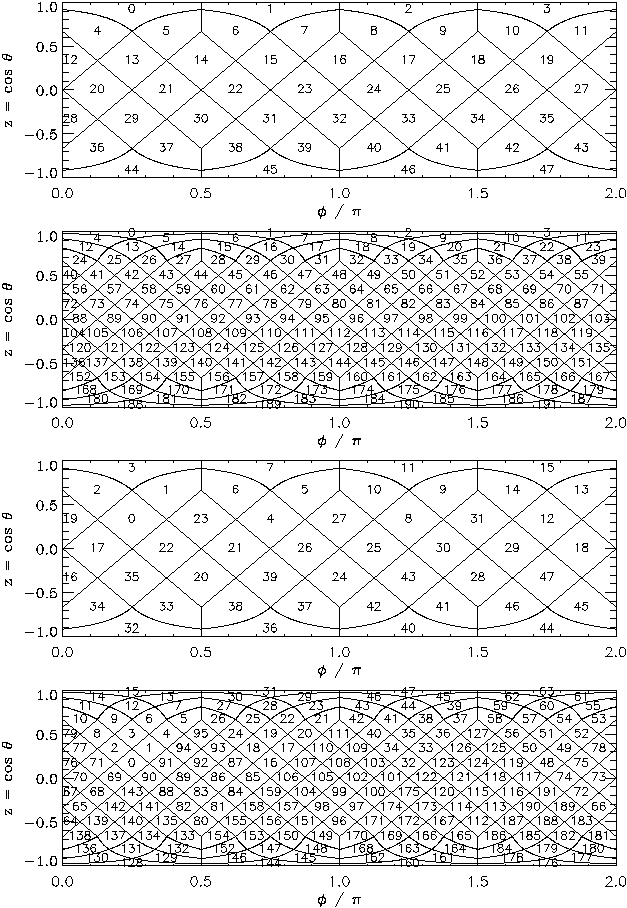
HEALPix RING and NESTED indexing schemes — The **RING** and **NESTED** indexing schemes of HEALPix. Reproduced from The image below, reproduced from [2].¶

There is a third HEALPix indexing scheme called UNIQ. The UNIQ indexing scheme is special because it encodes both the resolution and the sky position in a single integer. It assigns a single unique integer to every HEALPix tile at every resolution. If ipix is the pixel index in the NESTED ordering, then the unique pixel index uniq is:

\[\mathit{uniq} = \mathit{ipix} + 4 \, \mathit{nside}^2.\]

The inverse is:

\[\begin{split}\mathit{nside} = 2^{\lfloor \log_2(\mathit{uniq}/4)/2 \rfloor} \\ \mathit{ipix} = \mathit{uniq} - 4 \, \mathit{nside}^2.\end{split}\]

FITS Format for Multi-Order Sky Maps¶

The FITS format for LIGO/Virgo/KAGRA multi-resolution sky maps uses the UNIQ indexing scheme and is a superset of the FITS serialization for Multi-Order Coverage (MOC) maps specified by IVOA [4] as part of the Hierarchical Progressive Survey (HiPS) capability [3], notably used by Aladin for storing and display all-sky image mosaics.

Let’s download an example multi-order FITS file with curl:

$ curl -O https://emfollow.docs.ligo.org/userguide/_static/bayestar.multiorder.fits

Let’s look at the FITS header:

$ fitsheader bayestar.multiorder.fits
# HDU 0 in bayestar.multiorder.fits:
SIMPLE  =                    T / conforms to FITS standard
BITPIX  =                    8 / array data type
NAXIS   =                    0 / number of array dimensions
EXTEND  =                    T

# HDU 1 in bayestar.multiorder.fits:
XTENSION= 'BINTABLE'           / binary table extension
BITPIX  =                    8 / array data type
NAXIS   =                    2 / number of array dimensions
NAXIS1  =                   40 / length of dimension 1
NAXIS2  =                19200 / length of dimension 2
PCOUNT  =                    0 / number of group parameters
GCOUNT  =                    1 / number of groups
TFIELDS =                    5 / number of table fields
TTYPE1  = 'UNIQ    '
TFORM1  = 'K       '
TTYPE2  = 'PROBDENSITY'
TFORM2  = 'D       '
TUNIT2  = 'sr-1    '
TTYPE3  = 'DISTMU  '
TFORM3  = 'D       '
TUNIT3  = 'Mpc     '
TTYPE4  = 'DISTSIGMA'
TFORM4  = 'D       '
TUNIT4  = 'Mpc     '
TTYPE5  = 'DISTNORM'
TFORM5  = 'D       '
TUNIT5  = 'Mpc-2   '
PIXTYPE = 'HEALPIX '           / HEALPIX pixelisation
ORDERING= 'NUNIQ   '           / Pixel ordering scheme: RING, NESTED, or NUNIQ
COORDSYS= 'C       '           / Ecliptic, Galactic or Celestial (equatorial)
MOCORDER=                   11 / MOC resolution (best order)
INDXSCHM= 'EXPLICIT'           / Indexing: IMPLICIT or EXPLICIT
OBJECT  = 'MS181101ab'         / Unique identifier for this event
REFERENC= 'https://example.org/superevents/MS181101ab/view/' / URL of this event
INSTRUME= 'H1,L1,V1'           / Instruments that triggered this event
DATE-OBS= '2018-11-01T22:22:46.654437' / UTC date of the observation
MJD-OBS =    58423.93248442635 / modified Julian date of the observation
DATE    = '2018-11-01T22:34:49.000000' / UTC date of file creation
CREATOR = 'BAYESTAR'           / Program that created this file
ORIGIN  = 'LIGO/Virgo/KAGRA'         / Organization responsible for this FITS file
RUNTIME =     3.24746292643249 / Runtime in seconds of the CREATOR program
DISTMEAN=    39.76999609489013 / Posterior mean distance (Mpc)
DISTSTD =    8.308435058808886 / Posterior standard deviation of distance (Mpc)
LOGBCI  =    13.64819688928804 / Log Bayes factor: coherent vs. incoherent
LOGBSN  =    261.0250944470225 / Log Bayes factor: signal vs. noise
VCSVERS = 'ligo.skymap 0.1.8'  / Software version
VCSREV  = 'becb07110491d799b753858845b5c24c82705404' / Software revision (Git)
DATE-BLD= '2019-07-25T22:36:58' / Software build date
HISTORY
HISTORY Generated by calling the following Python function:
HISTORY ligo.skymap.bayestar.localize(event=..., waveform='o2-uberbank', f_low=3
HISTORY 0, min_inclination=0.0, max_inclination=1.5707963267948966, min_distance
HISTORY =None, max_distance=None, prior_distance_power=2, cosmology=False, mcmc=
HISTORY False, chain_dump=None, enable_snr_series=True, f_high_truncate=0.95)
HISTORY
HISTORY This was the command line that started the program:
HISTORY bayestar-localize-lvalert -N G298107 -o bayestar.multiorder.fits

This should look very similar to the FITS header for the standard HEALPix file from the previous section. The key differences are:

The ORDERING key has changed from NESTED to NUNIQ.
The INDXSCHM key has changed from IMPLICIT to EXPLICIT.
There is an extra column, UNIQ, that explicitly identifies each pixel in the UNIQ indexing scheme.
The PROB column has been renamed to PROBDENSITY, and the units have change from probability to probability per steradian.

Reading Multi-Resolution Sky Maps¶

Now let’s go through some of the same common HEALPix operations from the previous section, but using the multi-resolution format. Instead of Healpy, we will use astropy-healpix because it has basic support for the UNIQ indexing scheme.

First, we need the following imports:

>>> from astropy.table import QTable
>>> from astropy import units as u
>>> import astropy_healpix as ah
>>> import numpy as np

Next, let’s read the sky map. Instead of a special-purpose HEALPix method, we just read the FITS file into an Astropy table using Astropy’s unified file read/write interface:

>>> skymap = QTable.read('bayestar.multiorder.fits')

Most Probable Sky Location¶

Next, let’s find the highest probability density sky position. This is a three-step process.

Find the UNIQ pixel index of the highest probability density tile:

>>> i = np.argmax(skymap['PROBDENSITY'])
>>> uniq = skymap[i]['UNIQ']

What is the probability density per square degree in that tile?

>>> skymap[i]['PROBDENSITY'].to_value(u.deg**-2)
0.07825164701914111

Unpack the UNIQ pixel index into the resolution, nside, and the NESTED pixel index, ipix, using the method astropy_healpix.uniq_to_level_ipix(). (Note that this method returns level, which is the logarithm base 2 of nside, so we must also convert from level to nside using astropy_healpix.level_to_nside().)
```
>>> level, ipix = ah.uniq_to_level_ipix(uniq)
>>> nside = ah.level_to_nside(level)
```

Convert from nside and ipix to right ascension and declination using astropy_healpix.healpix_to_lonlat() (which is equivalent to hp.pix2ang):

>>> ra, dec = ah.healpix_to_lonlat(ipix, nside, order='nested')
>>> ra.deg
194.30419921874997
>>> dec.deg
-17.856895095545468

Probability Density at a Known Position¶

Now let’s look up the probability density at a known sky position. In this case, let’s use the position of NGC 4993:

>>> ra = 197.4133 * u.deg
>>> dec = -23.3996 * u.deg

Brute Force Linear Search

The following brute force method of looking up a pixel by sky position has a complexity of \(O(N)\), where \(N\) is the number of multi-resolution pixels.

Unpack the UNIQ pixel indices into their resolution and their NESTED pixel index.

>>> level, ipix = ah.uniq_to_level_ipix(skymap['UNIQ'])
>>> nside = ah.level_to_nside(level)

Determine the NESTED pixel index of the target sky position at the resolution of each multi-resolution tile.
```
>>> match_ipix = ah.lonlat_to_healpix(ra, dec, nside, order='nested')
```
Find the multi-resolution tile whose NESTED pixel index equals the target pixel index.
```
>>> i = np.flatnonzero(ipix == match_ipix)[0]
>>> i
13484
```
That pixel contains the target sky position. The probability density per square degree at that position is
```
>>> skymap[i]['PROBDENSITY'].to_value(u.deg**-2)
0.034679190989078075
```

Fast Binary Search

The following binary search method of looking up a pixel by sky position exploits the algebraic properties of HEALPix. It has a complexity of \(O(\log N)\) where \(N\) is the number of multi-resolution pixels. It assumes that every sky position is mapped on to exactly one multi-resolution tile, which is true for LIGO/Virgo/KAGRA multi-resolution sky maps.

First, find the NESTED pixel index of every multi-resolution tile, at an arbitrarily high resolution. (nside = 2**29 works nicely because it is the highest possible HEALPix resolution that can be represented in a 64-bit signed integer.)
```
>>> max_level = 29
>>> max_nside = ah.level_to_nside(max_level)
>>> level, ipix = ah.uniq_to_level_ipix(skymap['UNIQ'])
>>> index = ipix * (2**(max_level - level))**2
```
Sort the pixels by this value.
```
>>> sorter = np.argsort(index)
```

Determine the NESTED pixel index of the target sky location at that resolution.

>>> match_ipix = ah.lonlat_to_healpix(ra, dec, max_nside, order='nested')

Do a binary search for that value.

>>> i = sorter[np.searchsorted(index, match_ipix, side='right', sorter=sorter) - 1]
>>> i
13484

That pixel contains the target sky position. The probability density per square degree at that position is

>>> skymap[i]['PROBDENSITY'].to_value(u.deg**-2)
0.034679190989078075

Find the 90% Probability Region¶

Follow these steps to find the 90% probability region.

Sort the pixels of the sky map by descending probability density.
```
>>> skymap.sort('PROBDENSITY', reverse=True)
```

Find the area of each pixel.

>>> level, ipix = ah.uniq_to_level_ipix(skymap['UNIQ'])
>>> pixel_area = ah.nside_to_pixel_area(ah.level_to_nside(level))

Calculate the probability within each pixel: the pixel area times the probability density.
```
>>> prob = pixel_area * skymap['PROBDENSITY']
```
Calculate the cumulative sum of the probability.
```
>>> cumprob = np.cumsum(prob)
```
Find the pixel for which the probability sums to 0.9 (90%).
```
>>> i = cumprob.searchsorted(0.9)
```
The area of the 90% credible region is simply the sum of the areas of the pixels up to that one.
```
>>> area_90 = pixel_area[:i].sum()
>>> area_90.to_value(u.deg**2)
30.975181093574633
```

Save the 90% Probability Region Footprint as a MOC¶

Having found the 90% probability region, it’s easy to now write it out its footprint as a MOC suitable for visualization in Aladin.

Keep only the pixels that are within the 90% credible region.
```
>>> skymap = skymap[:i]
```
Sort the pixels by their UNIQ pixel index.
```
>>> skymap.sort('UNIQ')
```
Delete all columns except for the UNIQ column.
```
>>> skymap = skymap['UNIQ',]
```
Write to a FITS file.
```
>>> skymap.write('90percent.moc.fits')
```